Probability and Statistics

Central Limit Theorem

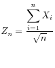
Central limit theorem. Let $X_1,X_2,\ldots$ be a sequence of independent uniform random variables on $(-\sqrt{3}, \sqrt{3})$ ; thus,

and $\textrm{Var}(X_i) = 1$ . Then

$\displaystyle Z_n = \frac{\displaystyle\sum_{i=1}^n X_i}{\sqrt{n}}$

converges to the standard normal distribution.

NN = c(1,2,5,100);
size = 1000;
intval = c(-sqrt(3), sqrt(3));
range = c(-3.4, 3.4);
breaks = seq(range[1], range[2], by=0.2);
x = seq(range[1], range[2], length=100);
y = dnorm(x);
par(mfrow=c(2,2));
for(n in NN){
  data = matrix(runif(n*size, intval[1], intval[2]), ncol=n);
  sample = apply(data, 1, sum) / sqrt(n);
  sample = sample[sample > range[1] & sample < range[2]];
  hist(sample, breaks, col='yellow', freq=F, main=paste("Simulated Distribution when n =", n));
  lines(x, y, type='l', lwd=2, col='blue');
}

Sample R code. You can download clt.R, and run it.

Problem 8. An actual voltage of new a -volt battery has the probability density function

$\displaystyle f(x) = 5, \quad 1.4 \le x \le 1.6.$

Estimate the probability that the sum of the voltages from

new batteries lies between

and

volts.

n = 120;
size = 10000;
range = c(170, 190);
data = matrix(runif(n*size, 1.4, 1.6), ncol=n);
sample = apply(data, 1, sum);
par(mfrow=c(2,1));
breaks = seq(range[1], range[2], by=0.25);
hist(sample, breaks, col=2, main="Distribution of Simulated Averages");
mean = 1.5 * n;
sd = sqrt((0.2^2/12) * n);
x = seq(range[1], range[2], length=100);
y = dnorm(x, mean, sd);
plot(x, y, type='l', lwd=1, frame.plot=F, main="Normal Approximation");

Problem 9. The germination time in days of a newly planted seed has the probability density function

$\displaystyle f(x) = 0.3 e^{-0.3 x}, \quad x \ge 0.$

If the germination times of different seeds are independent of one another, estimate the probability that the average germination time of

seeds is between

and

days.

rate = 0.3;
n = 2000;
size = 10000;
range = c(3, 3.7);
intval = c(3.1, 3.4);
data = matrix(rexp(n*size, rate), ncol=n);
sample = apply(data, 1, mean);
par(mfrow=c(2,1));
breaks = seq(range[1], range[2], by=0.025);
col = rep(0, length(breaks));
col[breaks >= intval[1] & breaks < intval[2]] = 2;
hist(sample, breaks, col=col, main="Distribution of Simulated Averages");
prop = length(sample[sample >= intval[1] & sample <= intval[2]]) / size;
text(intval[2], 10, prop);
mean = 1/rate;
sd = 1/(rate * sqrt(n));
x = seq(range[1], range[2], length=100);
y = dnorm(x, mean, sd);
plot(x, y, type='l', lwd=1, frame.plot=F, main="Normal Approximation");
x = seq(max(c(range[1],intval[1])),
        min(c(range[2],intval[2])), length = 50);
y = dnorm(x, mean, sd);
polygon(c(x,max(x),min(x)), c(y,0,0), col=2);
prob = pnorm(intval[2], mean, sd) - pnorm(intval[1], mean, sd);
text(intval[2], 0.1, round(prob,digits=4));

Sample R code. You can download problem8.R and problem9.R, and run them.